Lab: 7 Time Series Analysis
Written by Nicholas Coops
Lab Overview
In this lab, we will be using Landsat derived Best Available Pixel (BAP) imagery to examine changes in the Malcom Knapp Research Forest over a 19-year time span. In Task 1 you will use the “raster calculator” to calculate NDVI across the study area. In Task 2, you will use ArcPro to visualize a multidimensional NDVI data set and create a temporal profile. In task 3, you will conduct a change detection between two NDVI layers.
Learning Objectives
- Use Raster Functions tool to calculate NDVI in ArcGIS
- Interpret the physical meaning of regions of high, medium, and low NDVI
- Visualize temporal NDVI data in ArcGIS
- Create a temporal profile to help quantify changes in the image
- Use the change detection wizard to determine the difference in NDVI from 2000-2019
Data
The data for this lab consists of a Landsat derived BAP imagery from the year 2000 – 2019. Information on this dataset and direction for downloading similar datasets can be found here:
White, J.C.; Wulder, M.A.; Hobart, G.W.; Luther, J.E.; Hermosilla, T.; Griffiths, P.; Coops, N.C.; Hall, R.J.; Hostert, P.; Dyk, A.; et al. Pixel-based image compositing for large-area dense time series applications and science. Can. J. Remote Sens. 2014, 40, 192–212, doi:10.1080/07038992.2014.945827.
https://github.com/saveriofrancini/bap
Task 1: Calcualting NDVI from a Landsat image
Step 1: Start a new ArcGIS Pro Map project and drag-and-drop the MKRF_UTM10S_2019_BAP.tif file into the map window. At this point, you should see an RGB satellite image of the Malcolm Knapp Research Forest (Figure 7.1) if the map view does not immediately pan to the image right-click MKRF_UTM10S_2019_BAP.tif in the Contents pane and press Zoom to Layer.
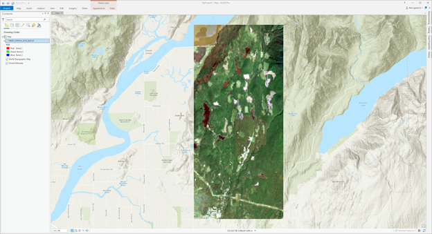
Figure 7.1: True colour composite of Malcom Knapp Research Forest (MKRF).
Best Available Pixel Composites: To date, you have worked with single Landsat images acquired at one time. Oftentimes, there can be clouds or haze that obstruct parts of an image and reduce the amount of usable data from a single image acquisition. Best Available Pixel Composites address this issue by combining multiple images taken at different times into an “image stack” and creating a new image using only the best cloud-free pixels from the image stack. For this lab you are using a BAP composite created from images taken over the 2019 peak growing season.
Q1. Why do you think BAP composites only use peak growing season imagery (July-August)? (5 points)
Step 2: Spectral indices are mathematical equations containing spectral reflectance values from two or more wavelengths used to highlight areas of spectral importance in an image. There are a wide variety of spectral indices used to highlight a variety of different land covers and image properties including burned Areas (Normalized Burn Ratio), urban/ built up areas (Normalized Difference Built-Up Index), and water (Normalized Difference Water Index) to name a few. The Normalized Difference Vegetation Index (NDVI) is a frequently used spectral index that takes advantage of the high near-infrared reflectance and high red absorption properties of healthy vegetation and is therefore often used to quantify vegetation in a remotely sensed multispectral image.
NDVI is calculated with the below formula:
\[ NDVI=\frac{NIR-Red}{NIR+Red} \] Where NIR is the near-infrared band (Landsat 7 Band 4) and Red is the red band (Landsat 7 Band 3). The results of this equation should be between -1 and 1 with values less than 0 representing water and values between 0-1 representing different levels of green vegetation.
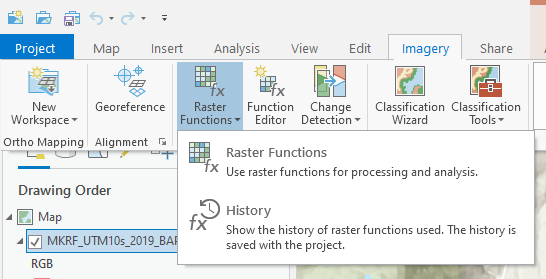
Navigate to the Imagery ribbon at the top of your ArcPro window and click the Raster Function button.
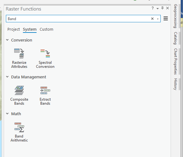
The Raster Functions pane should appear, you can either navigate the drop-down menus to “Math”, then “Band Arithmetic” or use the search function to find the Band Arithmetic Tool and click to open.
The “Band Arithmetic Properties” dialogue should appear. Under “Raster” use the drop-down menu and select the MKRF_UTM10s_2019_BAP.tif layer. If it is not currently in your map view and can use the folder button and navigate to your lab data folder and select the file. Under “Method” select User Defined. It should look like the screenshot below.
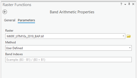
Use your knowledge of spectral indices and the NDVI formula given above to fill in the NDVI calculation for your data.
“Create new layer” at the bottom of the window. The output should look something like Figure 7.2.
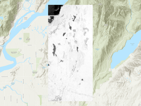
Figure 7.2: Example output for the 2019 NDVI raster calculation for MKRF
Task 2: Time Series Analysis
In the previous section of this lab you calculated NDVI for an image of the Malcom Knapp Research Forest. In this section you will use a multidimensional dataset containing NDVI layers from 2000-2019 to create a temporal profile of NDVI change over time.
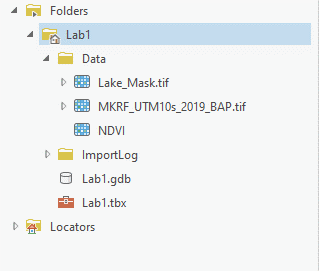
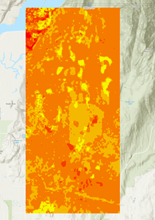
Open the Catalogue pane and navigate to the lab data folder. Click the arrow for the data folder to expand. Click and drag the NDVI multidimensional data set into your map viewer.
After opening the multidimensional dataset a new ribbon should appear at the top called Time along with a slider at the top of the map pane.
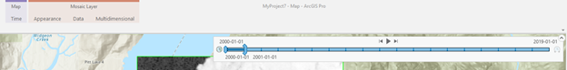
Press the play button on the slider to start an animation of NDVI change over time. You can also click and drag the slider to view individual years.
Q4. Hypothesize on what is causing the changes in NDVI? Why might the pattern in the south west corner of the timelapse look different from other changes? (15 points)
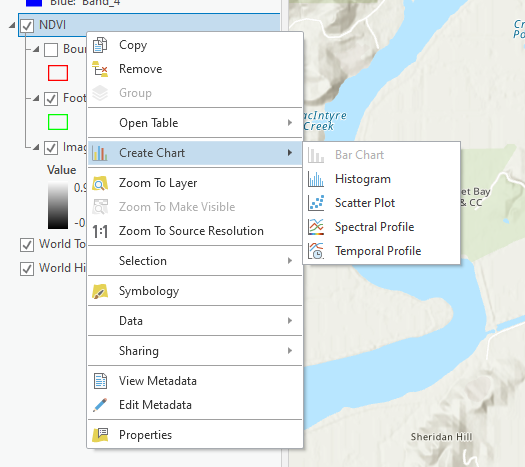
Now that you have visualized the imagery, it is time to create a temporal profile help quantify the changes in the images. Right-click on the NDVI layer in the Contents pane and hover over “Create Chart” and select Temporal Profile.
The “Temporal Profile” pane should appear on your screen, select “Properties” at the top of this pane. The “Chart Properties” pane should appear. Under “Time series” select “Multiple Locations with one variable” and select “Point” under area of interest.
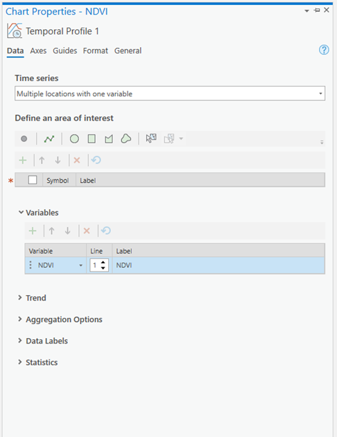
Your cursor should change into a coloured dot when hovering over the map pane. Clicking the left mouse button will select a pixel to view on your temporal profile. Use the Time slider animation function to find 4 changes that occur in different years, a 5th pixel representing water and a 6th representing an area with minimal change. See example bellow for possible locations but feel free to find and select your own.

Click “Export” in the Temporal profile pane and save your chart as a jpeg and submit it in your final report.
Task 3: Change Detection
Select the NDVI layer in the Contents pane, navigate to the Imagery ribbon and select Change Detection Wizard. A new pane should appear, under “Change Detection Method” select Pixel Value Change. Choose your NDVI multidimensional dataset as the “Input Raster”. “Variable” and “Dimension” should auto fill to NDVI and StdTime. Under “From Slice” select the year 2000 for “To Slice” select 2019 and press “Next”. In the next window select Absolute under “Difference Type” and leave the remainder as default and press “Next” at the bottom. The “Classify Difference” pane should appear and you should see a histogram. Uncheck the “Classify the difference in values” button and then press “Next”. Under “Smoothing Neighborhood” select 3x3 and set the “Statistics Fill Method” to median. Save your result as a raster dataset and under “Output Dataset” write “ChangeDetection_2000_2019” and press “Finish”.
Your results should appear in your map area. If you see a gray box right-click the layer in the Contents pane and select “Symbology”. Under Primary symbology use the drop-down menu and select Classify. You should now see an image on your screen that looks something like this:
This output shows the difference in NDVI values between the 2000 and 2019 values close to zero mean that no change occurred while negative values represent a decrease in NDVI and positive values an increase in NDVI.
Next, we will use the NDVI change layer to identify decreases in NDVI representing cut blocks.
We are now going to use Geoprocessing tools to extract only the areas that have been identified. Navigate to the Analysis tab and select “Tools”, then “Reclassify (Spatial Analyst Tools)”.
The “Reclassify Window” should appear. Under the reclassification table press the Classify button and under “Number of Classes” write 2. The table should change and look like this:
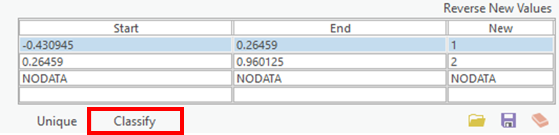
Change the “End” value in the first class to -0.05 and the “Start” value in the second class to -0.049999 and change the new field from 2 to NODATA. Run the tool. Your output should be a layer containing only pixels that had a negative change between the year 2000 NDVI image and the year 2019 NDVI image.
Notice that some of the pixels you have retained are lakes. Since we are principally concerned with terrestrial vegetation it is common practice to remove pixels that represent water using a water mask. Masking can either be done as a pre-processing step or at the end of our analysis.
Navigate to the “Analysis” ribbon and select Tools. Search for the tool “Extract by Mask”. Under “Input Raster” select your cutblock raster and under feature mask data navigate to the data folder and select the “LakeMask” file. Save your output as “NDVICutblocks” select run.
Summary
Spectral Indices offer a unique ability to highlight landcover and image properties that would be very difficult to map without the use of spectral information. The Normalized Difference Vegetation Index (NDVI) has become one of the most widely used indices and thanks to satellite programs like Landsat, we now have access to global coverage of this index. In this lab, we explored the ability to derive this index from Landsat BAP data from 2000-2019 in ArcGIS and explore the temporal profile of NDVI to quantify changes in the image through time. We can use change detection tools to then be able to assess regions that have changed significantly through our time period. Time series data of spectral indices like NDVI can be game changing for many research applications like monitoring drought, agricultural productivity, and measuring biomass! Return to the Deliverables section to check off everything you need to submit for credit in the course management system.