Show the code
## develop a sample
plot_sample <- sample(x = 1:112, size = 15, replace = F)Written by
This lab uses a “simulated” forest to practice simple random sampling, summarizing the data, and then using that information as we would in a real forest environment. We will use this sample data to estimate important forest metrics and confidence around our estimates.
Estimate the population mean and the confidence intervals using simple random sampling
Apply estimates + confidence intervals to answer management questions
Apply a systematic sampling design to estimate population mean and confidence intervals
Compare the cost and relative efficacy of different sampling regimes.
Prior to completing this exercise go over the terminology and equations included the course lecture material. It is important to know what a population mean is and how we describe this using estimators
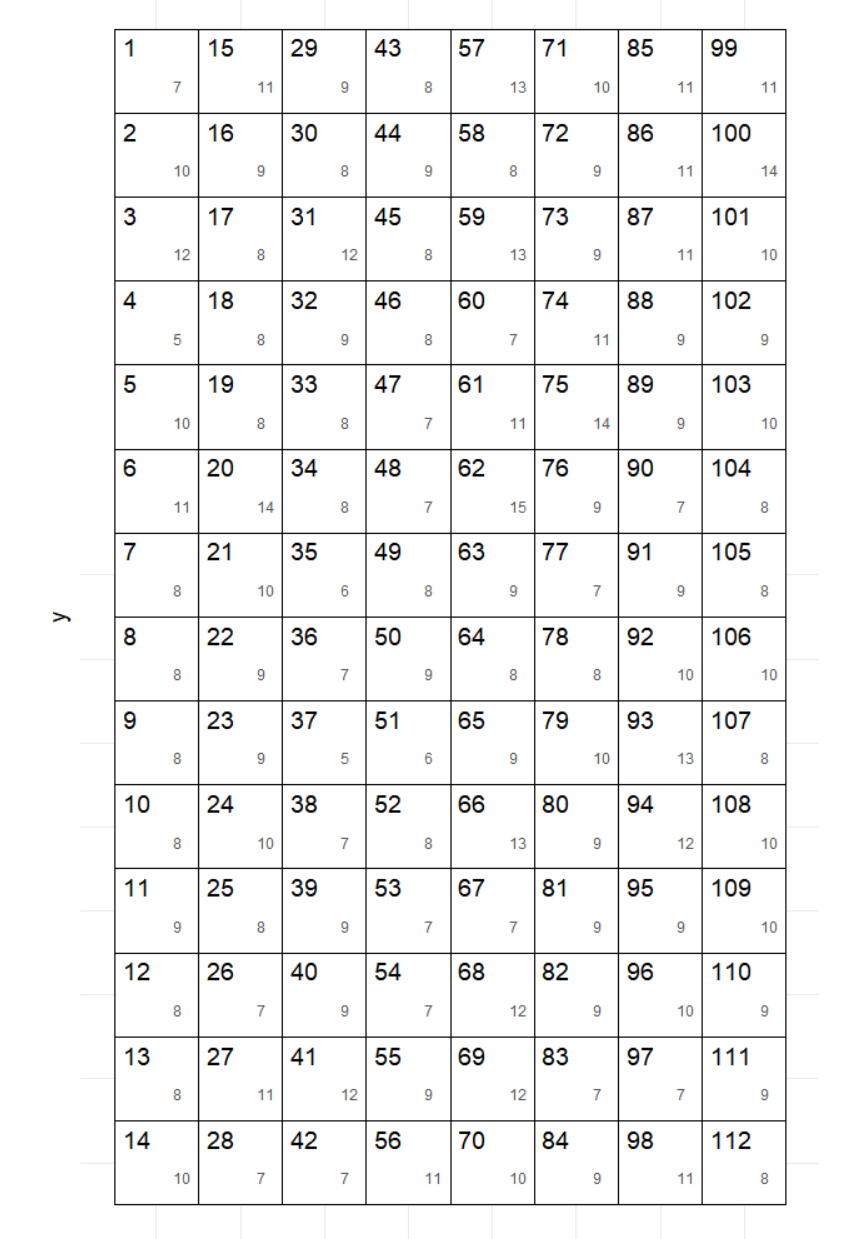
Simulated Forest Landscape
Step 1
Using the map above select n=15 plots using simple random sampling without replacement. Explain how you used simple random sampling replacement to select the data. How did you choose random numbers?
## develop a sample
plot_sample <- sample(x = 1:112, size = 15, replace = F)Calculate:
You must should calculations and include measurement units in your responses. For your confidence interval calculation, shot is a range with the lower value first.
Convert the estimated mean volume per plot and the associated confidence interval to an equivalent per hectare estimate (e.g. 200m3/ha with a confidence interval of (100 m3/ha)
Based on the volume per ha values, where in BC might these data have come from? Consider (1) ecosystem type (2) time since disturbances. To provide context, a very productive old stand in the Boreal Forest of Canada could have up to 500 m3/ha (most are much less). A very productive old stand in the Temperate Rainforest of the western coast of Canada could have 1,500 m3/ha. Also, 1 m3 is about the size of a utility pole (e.g., telephone or electricity pole).
How large is total plot area in hectares (you determined this in Activity 3 already)? Use this to expand the mean in m3/ha and the associated confidence interval to obtain the estimated total m3 volume for the land area and a 95% confidence interval for this estimate. Based on this confidence interval, would you say that there could be 1200 m3 of volume in this area?
Calculate the Percent Error achieved for your survey. Did you achieve the desired percent error of + or – 15% of the mean with 95% probability? NOTE: This is the standard for operational cruising in BC for scale-based sales (i.e., billing is based on scaled logs not on standing estimated cruise volumes).
For the following questions imagine a forester is planning a survey with the with the following specifications:
Intensity (I) = 0.02 (i.e., 2 %)
Forest land area (A) = 100 ha (1000 m X 1000 m; 1 ha = 10,000 m2)
Size of plot (a)= 0.02 ha (i.e., 14.14 X 14.14 square plot)
The area of the all of the plots of that will be needed for this forester’s survey using this intensity (Ap); and
The number of samples (n) required for this desired sampling intensity, given the specified plot size.
Given that the length between plot centres (B) is fixed at 40 m, what is the length between lines (L)? NOTE: In practice, we would round down to the nearest 5 m to lay this out in the field. For example, if the answer was 103 m, we would use 40 m by 100 m spacing (not 105 m and not 103 m spacing), since forest land areas are often irregular in shape and this would “pull in” the systematic sampling grid to hopefully get enough plots.
What would the spacing be, if this square spacing between plot centres was used instead? Again, in practice, we would round this answer down to the nearest 5 m to lay this out in the field.
Which of these two options would you choose to use and why?
Using the square spacing calculated in 2b and the plot size, select random co-ordinates for you first plot centre in the first “grid” of your systematic survey. Show all calculations you used to get the random co-ordinates and to make sure that the plot will fit within the first “grid square” of your systematic survey given these random co-ordinates and the plot dimensions.
Given a fixed project cost of $5,000 (i.e., truck rental and other equipment) and a per day cost of $1,000 for a 2-person crew with a production rate of eight plots per day:
How long would the survey take?
What would the cost of this survey be?
if the budget was set at $10,000:
How many plots could you have measured using the cost estimates in #10?
What would the sampling intensity be for this fixed budget?
Would this sampling intensity be more or less than the sampling intensity used in the sample plan (i.e., planned for 2%)?
In this lab, we practiced the calculations of important summary statistics from a random sampling design. We also learned and applied our investigation to look at sampling intensity in systematic random sampling.